The Global CO2 Distribution product provides a visual representation of CO2 mole fractions based on global 2.0×2.0° grids as numerically estimated using observation data from around 150 sites worldwide.
Observation data and numerical modelling of atmospheric transport allow estimation of CO2 mole fractions for various areas over extended periods including regions for which there are no observation data. In particular, Global CO2 Distribution provides information on CO2 mole fractions in upper-air regions where there are no data except for a small number of aircraft observation results.
The analysis method and related accuracy are described below, with further details provided in the articles listed at the bottom of the page.
CO2 flux serves as a fundamental quantity in the numerical analysis, and is defined as the amount of CO2 passing by a unit area of ground or sea surface in a unit time. The change in the amount of CO2 at one point on the surface will be reflected, via the transport of CO2 by wind, in CO2 mole fractions over an extensive region, including upper-air spaces. In other words, the CO2 mole fraction for a particular time and place is evaluated as the sum of the influences of all fluxes under consideration. Calculation of this process is governed by an atmospheric transport model that describes the transport of CO2 by wind. In this work, the model GSAM-TM (Nakamura et al., 2015) is adopted.
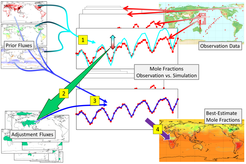
To prevent estimated mole fractions from being unrealistic, three prior fluxes concerning human activity, the terrestrial biosphere and oceans are produced in consideration of various studies on CO2 emission and uptake. Based on these data, the atmospheric transport model makes an initial estimate of mole fractions for every grid point and time step of simulation (1). As the resulting mole fractions generally do not correspond to actual observation values, the compensation procedure outlined below is carried out.
With the whole globe divided into a number of prescribed regions, the atmospheric transport model estimates how a monthly unit amount of flux allocated to each region influences mole fractions for every grid point and time step. A coefficient is then determined for each unit flux so that the set of fluxes multiplied by the coefficients best compensates for the correspondence mismatch stated above. In determination of the coefficient set, uncertainties in prior fluxes and observed mole fractions are appropriately considered. This approach is known as the inversion method (2 3).
Based on the prior fluxes and the fluxes determined using the inversion method described above, CO2 mole fractions are finally determined for every grid point and time step, and the outcomes are used to create the Global CO2 Distribution product (4).
Nakamura et al. (2015) compared numerical results with observation data from the CONTRAIL* project that are not adopted in the analysis, and found that the root mean square difference was around 3 ppm from the surface to a height of 1 km and around 1 ppm at a height of 6 km.
The authors are grateful to all contributors for permission to use the relevant data. This work is supported by the National Science Foundation (OCE-9900310), the National Oceanic and Atmospheric Administration (NA67RJ0152, Amendment 30), the Global Analysis, Interpretation, and Modeling Project of the International Geosphere Biosphere Program, and the Global Carbon Project. Thanks also go to R. Law, K. Gurney and P. J. Rayner for providing the TDI model codes.
Maki, T., M. Ikegami, T. Fujita, T. Hirahara, K. Yamada, K. Mori, A. Takeuchi, Y. Tsutsumi, K. Suda and T.J. Conway, 2010: New technique to analyse global distributions of CO2 concentration and fluxes from non-processed observational data. Tellus B, 62 (5), 797 – 809, https://doi.org/10.1111/j.1600-0889.2010.00488.x.
Nakamura, T., T. Maki, T. Machida, H. Matsueda, Y. Sawa and Y. Niwa, 2015: Improvement of Atmospheric CO2 Inversion Analysis at JMA. A31B-0033 (https://agu.confex.com/agu/fm15/meetingapp.cgi/Paper/64173), AGU Fall Meeting, San Francisco, 14 – 18 Dec. 2015.