Before you start, you need download One-month Prediction GPV data file from here, and convert that file into GrADS file. ( See "To convert a GRIB2 format file at TCC into GrADS format" for Linux for windows )
* Lesson 1 : start up GrADS / open file / draw a picture
To start up GrADS, enter:
grads
If grads is not in your current directory, or if it is not in your PATH somewhere, you may need to enter the full pathname, ie:
/usr/homes/smith/grads/grads
GrADS will prompt you with a landscape vs. portrait question; just press enter. At this point a graphics output window should open on your console. You may wish to move or resize this window. Keep in mind that you will be entering GrADS commands from the window where you first started GrADS -- this window will need to be made the 'active' window and you will not want to entirely cover that window with the graphics output window.
In the text window (where you started grads from), you should now see a prompt: ga-> You will enter GrADS commands at this prompt and see the results displayed in the graphics output window.
The first command you will enter is:
open mg1w.ctl
You may want to see what is in this file, so enter:
query file
One of the available variable is called ps, for sea-level pressure. We can display this variable by entering:
d psead is short for display. You will note that by default, GrADS will display an X, Y plot at the first time and at the lowest level in the data set.
* Lesson 2 : change dimension environment
clear           clears the display
set lon 90      sets longitude to 90 degrees East
set lat 40      sets latitude to 40 degrees North
set lev 1       sets level to 1 (* just one level is available now. )
set t 1         sets time to first time step
d z500          displays the variable 'z500'
In the above sequence of commands, we have set all four GrADS dimensions to a single value. When we set a dimension to a single value, we say that dimension is "fixed". Since all the dimensions are fixed, when we display a variable we get a single value, in this case the value at the location 90E, 40N, (lev=1), and the 1st time in the data set. See "Result value = ???"
clear
set lon 0 180     X is now a varying dimension
d z500
We have set the X dimension, or longitude, to vary. We have done this by entering two values on the set command. We now have one varying dimension (the other dimensions are still fixed), and when we display a variable we get a line graph, in this case a graph of 500mb Heights at 40N.
clear
set lat 0 90
d z500
We now have two varying dimensions, so by default we get a contour plot.
c
set t 1 4
d z500
we get an animation sequence, in this case through time.
clear
set lon 0 360
set lat 0 90
set t 1
d psea
d z500
In this case we have also displayed two variables, which simply overlay each other. You may display as many items as you desire overlaid before you enter the clear command.
c
set lon 0 360
set lat 40
set t 1 4
d z500
* Lesson 3 : use operators and functions
clear
set lon 0 180
set lat 0 90
set lev 1
set t 1
display (t850-273.16)*9/5+32
clear
d sqrt(u850*u850+v850*v850)
to calculate the magnitude of the wind. A function is provided to do this calculation directly:
d mag(u850,v850)
clear
d ave(z500,t=1,t=4)
In this case we calculate the 4 week mean.
We can also remove the mean from the current field:
clear
d z500 - ave(z500,t=1,t=4)
We can also take means over longitude to remove the zonal mean:
clear
d z500-ave(z500,x=1,x=144)
clear
d z500(t=2)-z500(t=1)
This computes the change between the two fields over 1 week. We could have also done this calculation using an offset from the current time:
clear
d z500(t+1) - z500
clear
d hcurl(u850,v850)
* Lesson 4 : controll the graphics output
clear
set cint 30
d z500
clear
set ccolor 3
d z500
clear
set gxout shaded
d hcurl(u850,v850)
This is not very smooth; we can apply a cubic smoother by entering:
clear
set csmooth on
d hcurl(u850,v850)
set gxout contour
set ccolor 0
set cint 30
d z500
draw title 500hPa Height and 850hPa Vorticity
clear
set gxout vector
d u850;v850
clear
d u850;v850;rain
or maybe:
clear
d u850;v850;hcurl(u850,v850)
clear
d mag(u850,v850) ; rain*0.1
Here the U component is the wind speed; the V component is precipitation.
clear
set gxout stream
d u850;v850;hcurl(u850,v850)
clear
set gxout grid
d u850
clear
set lon 70 110
set lat 30 45
set digsize 0.2
d u850
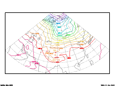
clear
set lon 40 140
set lat 15 80
set mproj nps
set gxout contour
set cint 30
d z500
printim fig01.gif x800 y600 blackIn this case, the "printim" command produces a GIF formatted image file on the current contents displayed on the screen, which has a resolution of 800x600 using black background.
You can make a PNG formatted image file and change background and resolution if you want.
printim fig02.png x400 y300 white
This concludes the sample session. At this point, you may wish to examine the data set further, or you may want to go through the GrADS documentation and try out the other options described there.
| updated : Jun.30, 2004 | [ back ] |