This page provides download links to grid data on CO2 mole fractions used for the Global CO2 Distribution product.
The data stem from numerical analysis performed by JMA using observation data reported to the WMO World Data Centre for Greenhouse Gases (WDCGG). Any usage should be accompanied by the following citation.
Nakamura, T., T. Maki, T. Machida, H. Matsueda, Y. Sawa and Y. Niwa, 2015: Improvement of Atmospheric CO2 Inversion Analysis at JMA. A31B-0033 (https://agu.confex.com/agu/fm15/meetingapp.cgi/Paper/64173), AGU Fall Meeting, San Francisco, 14 – 18 Dec. 2015.
The horizontal resolution of the grid data was increased from 2.5° × 2.5° to 2.0° × 2.0° (latitude × longitude) on 27 February 2020.
Column-average CO2 mole fraction data from 7 March 2024 onward are available.
Each data file below contains monthly mean values of dry-air mole fractions (in units of ppm) for every 2.0° latitude × 2.0° longitude grid worldwide covering the 12 months of the year (as indicated by the file names), or those of column-average mole fractions covering the whole analysis period. The files are zip-compressed in NetCDF format.
In regard to monthly mean values of dry-air mole fractions for each year, there are two data files with different descriptions of the vertical direction. One has nine constant pressure altitudes from the surface to a height of 8 km at 1 km intervals, and the other has 60 layers with σ-pressure hybrid coordinates.
The dimensions and variables of data with constant altitudes are shown below.
dimensions:
	time = 12 ;
	altitude = 8 ;
	latitude = 91 ;
	longitude = 180 ;
variables:
	int time(time) ;
		time:units = "months since 2022-01-16" ;
	int altitude(altitude) ;
		altitude:standard_name = "altitude" ;
		altitude:units = "m" ;
		altitude:axis = "Z" ;
		altitude:positive = "up" ;
	float latitude(latitude) ;
		latitude:units = "degrees_north" ;
	float longitude(longitude) ;
		longitude:units = "degrees_east" ;
	float co2_conc(time, altitude, latitude, longitude) ;
		co2_conc:units = "ppm" ;
		co2_conc:long_name = "Monthly mean grid CO2 mole fraction" ;
		co2_conc:missing_value = -999 ;
	float p_surf(time, latitude, longitude) ;
		p_surf:units = "Pa" ;
		p_surf:long_name = "Monthly mean surface pressure" ;
	float co2_surf(time, latitude, longitude) ;
		co2_surf:units = "ppm" ;
		co2_surf:long_name = "Monthly mean grid CO2 mole fraction (surface)" ;
The dimensions and variables of data with layers in σ-pressure hybrid coordinates are shown below.
In σ-pressure hybrid coordinates, pressure p(k) [hPa] at the lower surface of the k-th layer is determined using
p(k) = ak(k) + bk(k) * p_surf,
where p_surf is the surface pressure and ak(k) and bk(k) are conversion parameters. The values of p_surf, ak(k) and bk(k) are stored in the data files.
dimensions:
	time = 12 ;
	level = 60 ;
	latitude = 91 ;
	longitude = 180 ;
variables:
	int time(time) ;
		time:units = "months since 2022-01-16" ;
	int level(level) ;
		level:standard_name = "atmosphere_hybrid_sigma_pressure_coordinate" ;
		level:units = "level" ;
		level:axis = "Z" ;
		level:positive = "up" ;
		level:formula_terms = "ap: ak b: bk ps: p_surf" ;
	float ak(level) ;
		ak:long_name = "coeffient of vertical coordinate system" ;
		ak:units = "hPa" ;
	float bk(level) ;
		bk:long_name = "coeffient of vertical coordinate system" ;
	float latitude(latitude) ;
		latitude:units = "degrees_north" ;
	float longitude(longitude) ;
		longitude:units = "degrees_east" ;
	float co2_conc(time, level, latitude, longitude) ;
		co2_conc:units = "ppm" ;
		co2_conc:long_name = "Monthly mean grid CO2 mole fraction" ;
	float p_surf(time, latitude, longitude) ;
		p_surf:units = "hPa" ;
		p_surf:long_name = "Monthly mean surface pressure" ;
The dimensions and variables of data are shown below.
dimensions:
	lon = 180 ;
	lat = 91 ;
	time = UNLIMITED ; // (456 currently)
variables:
	double lon(lon) ;
		lon:standard_name = "longitude" ;
		lon:long_name = "longitude" ;
		lon:units = "degrees_east" ;
		lon:axis = "X" ;
	double lat(lat) ;
		lat:standard_name = "latitude" ;
		lat:long_name = "latitude" ;
		lat:units = "degrees_north" ;
		lat:axis = "Y" ;
	double time(time) ;
		time:standard_name = "time" ;
		time:units = "months since 1985-01-01 00:00:00" ;
		time:calendar = "standard" ;
	float xco2(time, lat, lon) ;
		xco2:long_name = "Monthly mean column-average CO2 mole fraction (XCO2) [ppm]" ;
		xco2:_FillValue = -9.99e+33f ;
		xco2:missing_value = -9.99e+33f ;
NetCDF format can be simply handled with the GrADS∗ program. Provided below are two sample GrADS scripts to demonstrate simple operation using the file 3D_concentration_L9_2022.nc.
∗The free Grid Analysis and Display System (GrADS) program is developed and distributed by the Center for Ocean-Land-Atmosphere Studies (COLA).
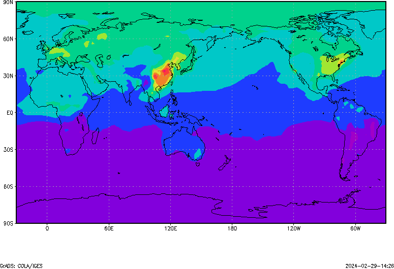
Sample 1 shows color-shaded contours for global surface CO2 mole fractions for January 2022.
sdfopen 3D_concentration_L9_2022.nc
set lat -90 90
set lon -30 330
set time Jan2022
set gxout shaded
d co2_surf
Sample 2 shows numerical values of CO2 mole fractions over 6 × 6 grid points from 30 to 40°N and from 130 to 140°E at a height of 6 km for January 2022.
sdfopen 3D_concentration_L9_2022.nc
set lat 30 40
set lon 130 140
set lev 6000
set time Jan2022
set gxout print
set prnopts %5.1f 6 1
d co2_conc
Printing Grid -- 36 Values -- Undef = -9.99e+08
418.2 418.1 418.1 418.1 418.0 418.0
418.8 418.8 418.7 418.7 418.7 418.7
419.3 419.3 419.3 419.3 419.4 419.4
419.8 419.8 419.7 419.7 419.6 419.6
419.9 419.8 419.8 419.8 419.8 419.8
419.7 419.7 419.8 419.8 419.8 419.9
Maki, T., M. Ikegami, T. Fujita, T. Hirahara, K. Yamada, K. Mori, A. Takeuchi, Y. Tsutsumi, K. Suda and T.J. Conway, 2010: New technique to analyse global distributions of CO2 concentration and fluxes from non-processed observational data. Tellus B, 62 (5), 797 – 809, https://doi.org/10.1111/j.1600-0889.2010.00488.x.
Nakamura, T., T. Maki, T. Machida, H. Matsueda, Y. Sawa and Y. Niwa, 2015: Improvement of Atmospheric CO2 Inversion Analysis at JMA. A31B-0033 (https://agu.confex.com/agu/fm15/meetingapp.cgi/Paper/64173), AGU Fall Meeting, San Francisco, 14 – 18 Dec. 2015.