Introduction

The Meteorological Satellite Center of the Japan Meteorological Agency (JMA/MSC) contributes to the Global Space-based Inter-Calibration System (GSICS) and examines ways to improve vicarious calibration for visible and near-infrared (VIS/NIR) bands of instrumentation on geostationary orbit (GEO) satellites. Under the GSICS framework, various ways of validating VIS/NIR-band sensor sensitivity are considered.
One such method, known as ray-matching, involves using the sensor on the Low Earth Orbit (LEO) satellite as reference for comparison against GEO instrument-based observation. As the reference sensor is well calibrated and stable, the bias of GEO observation can be estimated and correction values derived.

JMA/MSC plans to implement validation of Himawari-8/-9 VIS/NIR data based on the ray-matching technique with VIIRS as reference, in addition to the current validation based on radiative transfer simulation (RSTAR) data. This method has the following advantages over the existing approach:

No dependence on the radiative transfer model

Wide dynamic range with applied targets from low-reflectance (e.g., clear sky ocean) to high-reflectance (e.g., deep convective cloud)

Figure 1 outlines the JMA/MSC ray-matching process, and the items are subsequently described in detail.

Outcomes

The outcomes of the ray-matching approach are linear regression coefficients, scatter plots for individual bands, statistical CSV files and time-series graphs.

Coefficients of regression between reference and GEO imager observation

Regression coefficients are displayed as scatter plots and stored in CSV files (described later). Linear regression via the origin (referred to as force-fit regression) and with offsetting are applied. A regression coefficient (Slope) can be applied in force-fit regression using the equation below to produce corrected AHI reflectance (R_{corr_AHI}) in reference to VIIRS reflectance. R_{corr_AHI} = R_{org_AHI} / Slope .

Here, R_{org_AHI} is the original AHI reflectance.

Scatter plots

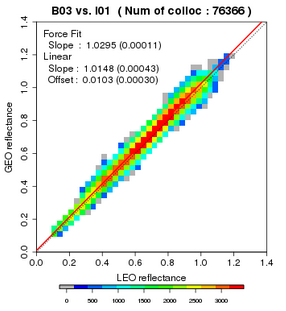
Fig. 2: Relationship between            Band 03 of AHI and I01 of VIIRS

Figure 2 shows the reflectance relationship between reference values based on SNPP/VIIRS and HIMAWARI-8/AHI.
Warm colors (e.g., orange, red) and cold colors (e.g., blue, grey) represent high and low numbers of collocations, respectively, and the coefficients for force-fit and linear regression are shown in the upper left. Values in parentheses represent standard errors. For simplicity, only the force-fit regression line is displayed (red line).

CSV files

Ray-matching results are also stored in CSV file format, including slope, offset and statistics based on both regression methods.

Time-series representation

Time-series graphs consist of three parts (Fig. 3), with the upper and middle ones showing offset and the slope of linear regression since July 2015, respectively. Red and blue plots represent statistics for t - 14 days to t + 14 days and for t + 0 days (t: date of validity), respectively. The bottom part shows collocation variations, with red bars representing half the number of collocation data gathered during the 29 days and blue bars representing the number of pixels gathered on the specific single day.

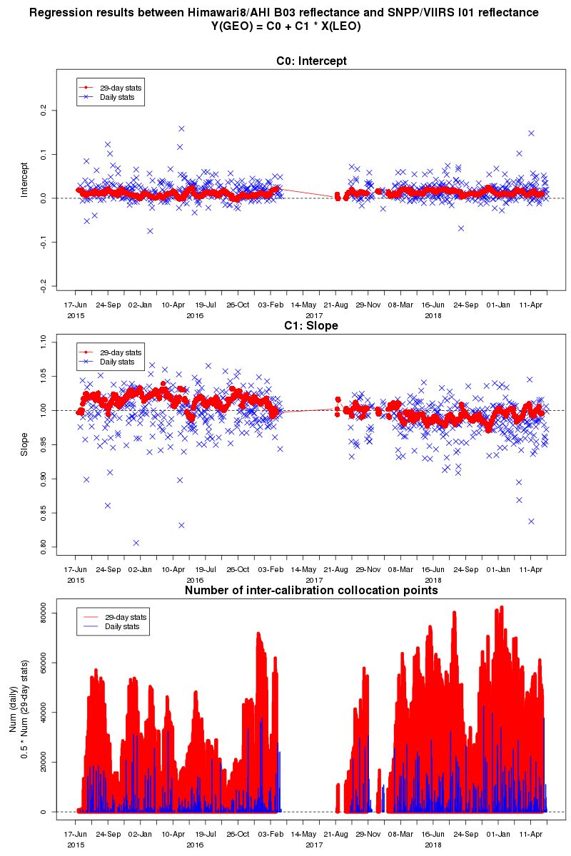Fig. 3: Time-series representations of slope, offset and numbers of collocations

Methodology

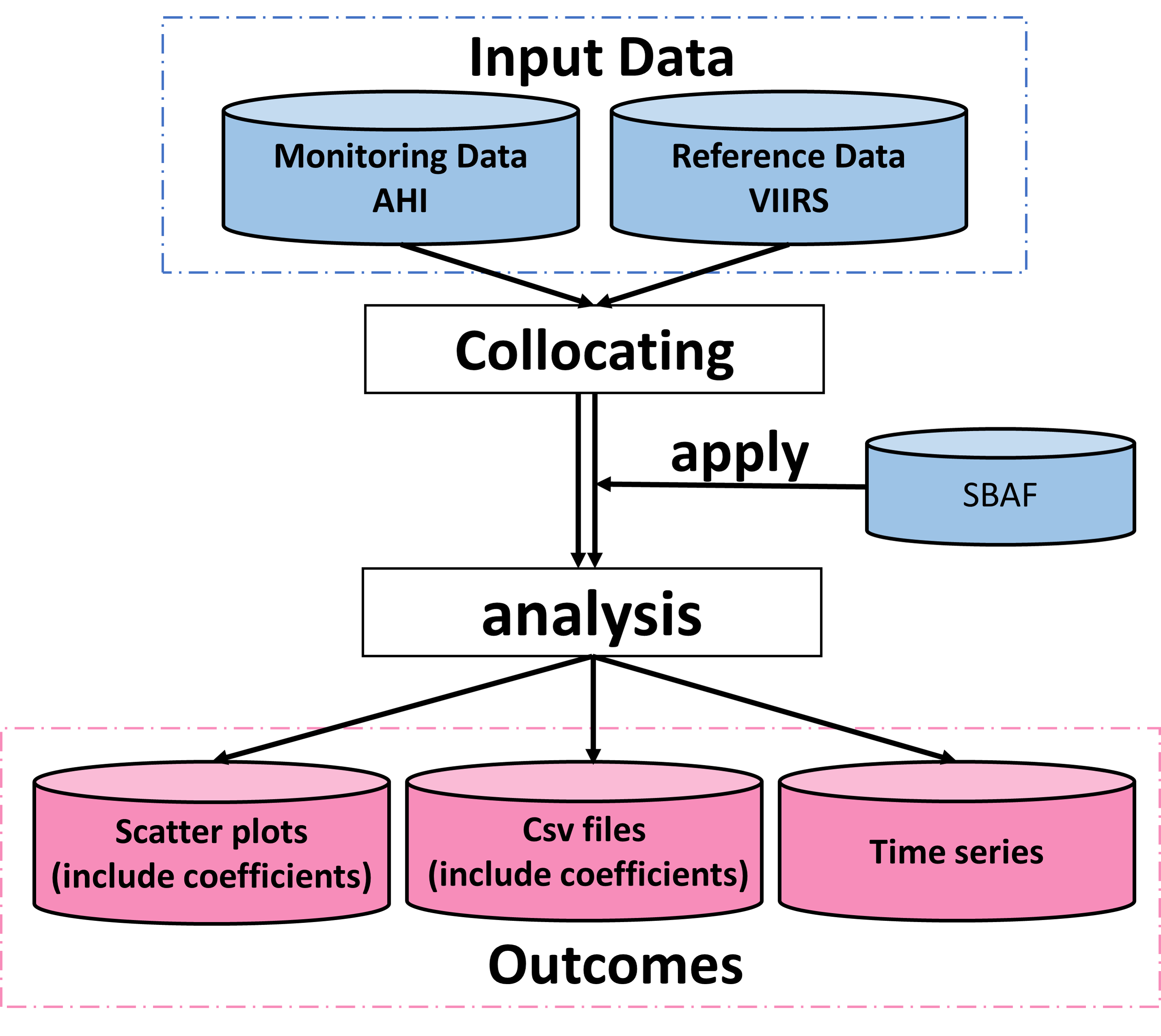
VIIRS data are used as reference for ray matching, and the reflectance of the AHI VIS/NIR bands is validated (Fig. 1).

Input

• Monitoring data: AHI
Himawari Standard Data (HSD) resampled with a spatial resolution of approximately 2 km at the sub-satellite point are used, with AHI reflectance calculated as Reflectance = Radiance × π d²/ F₀ cos(SZA)    (2) Here, d is the Earth-sun distance in AU (Astronomical Units) and F₀ is solar incident irradiance (see Table 1 of see the Visible and Near-Infrared Vicarious Calibration Guide), and cos(SZA) is the cosine of the solar zenith angle.

• Reference data: VIIRS
S-NPP and NOAA20/VIIRS SDR data from the NOAA class server are used for reference (Table 1: band details). Although the center wavelengths of VIIRS and AHI are similar for each band, their spectral response functions (SRFs) differ slightly. The difference is considered via a spectral band adjustment factor (SBAF) as described later. As the spatial resolutions of VIIRS and AHI data differ, VIIRS data pixels are averaged with surrounding pixels (M-band: 3 x 3 pixels; I-band: 5 x 5 pixels).

Collocation

From AHI and VIIRS data, pixels meeting the geometric conditions (Table 2) are extracted. AHI and VIIRS collocation data are produced by matching data with same positions.

Spectral band adjustment factors (SBAFs)

SBAFs are applied in ray-matching to correct slight differences in AHI and VIIRS spectral responses using NASA' web-based SBAF Tool. SBAFs are derived using Scanning Imaging Absorption Spectrometer for Atmospheric Chartography (SCIAMACHY) data and AHI/ VIIRS SRF values. Table 3 shows SBAFs between scaled radiance for AHI and VIIRS with the “Force Fit” and “All-sky Tropical Ocean” conditions set by NASA’s SBAF tool. As AHI Band 06 (2.3µm) is not supported by the tool, the SBAF of this band vs. VIIRS M11 is estimated via radiative transfer simulation using RSTAR.

For each band, SBAF is applied as

R_SBAF = SBAF × R_original Here, R_SBAF is VIIRS reflectance corrected using SBAF, and R_original is the original VIIRS reflectance in the SDR.

Comparison and monitoring

AHI reflectance is compared to VIIRS reflectance corrected using SBAF via linear regression, and the outcomes described above are derived.

Reference

• Ray-matching
  Doelling D., R. Bhatt, D. Morstad, B. Scarino, 2011: Algorithm Theoretical Basis Document (ATBD) for ray-matching technique of calibrating GEO sensors with Aqua-MODIS for GSICS (PDF, 302 kB)
  
  
• SBAF
  Scarino B. R, D. R. Doelling, P. Minnis, A. Gopalan, T. Chee, R. Bhatt, C. Lukashin, C. O. Haney, 2016: A web-based tool for calculating spectral band difference adjustment factors derived from SCIAMACHY hyperspectral data, IEEE Trans. Geosci. Remote Sens., 54, No. 5, 2,529 - 2,542
  
  
• RSTAR
  Nakajima, T., M. Tanaka, 1986: Matrix formulation for the transfer of solar radiation in a plane-parallel scattering atmosphere, J. Quant. Spectrosc. Radiat. Transfer, 35, 13 - 21
  Nakajima, T., M. Tanaka, 1988: Algorithms for radiative intensity calculations in moderately thick atmospheres using a truncation approximation, J. Quant. Spectrosc. Radiat. Transfer, 40, 51 - 69
  Stamnes, K., S.-C. Tsay, W. Wiscombe, K. Jayaweera, 1988: Numerically stable algorithm for discrete-ordinate-method radiative transfer in multiple scattering and emitting layered media, Appl. Opt., 27, 2,502 - 2,509