This page describes 1. Earthquakes and 2. Crustal strain in the upper layer.
The table shown here lists numbers of high-precision hypocenters (table, Section 1.2.3) in and around Japan along with selected low-precision hypocenters with a seismic intensity of 1 or more in Japan by region and magnitude. The Unknown column shows the number of earthquakes whose magnitude could not be determined, and the total number of quakes felt (measuring 1 or more on JMA's seismic intensity scale) is displayed at the bottom. District names for epicenters are based on the specifications of Appendix 1.A.3.. Tremors with a "Near Japan" district designation occurred in regions from No. 311 to No. 341, including Sakhalin, the Kurile Islands, the Korean Peninsula, the Ogasawara Islands, Primorskii and Taiwan.
The earthquake parameters in this bulletin are determined by JMA and agencies in other countries.
Hypocenters are calculated using P-wave and S-wave arrival times, and magnitudes are determined using maximum seismic wave amplitudes. Lists of seismic stations and standard seismograph response curves are shown in Appendices 1.A.1. and 1.A.2.,respectively.
| For P-waves ( Wp ) | Wp = Rmin 2/R 2 |
| For S-waves ( Ws ) | Ws = Wp/3 |
| Rmin : Hypocentral distance from the station nearest the hypocenter (km) | |
| ( if Rmin ≤ 50, Rmin = 50; if Wp > 1,Wp = 1) | |
Data from stations displaying large travel time residuals are not used for calculation. The depth of focus is initially calculated with no restrictions. If the solution for earthquake parameters is unstable, the best solution is sought with the epicenter fixed and the depth changed in increments of 1 km. For earthquakes located in the shallow region around the Kurile Islands (see Figure 1), the focal depth is fixed at 30 km.
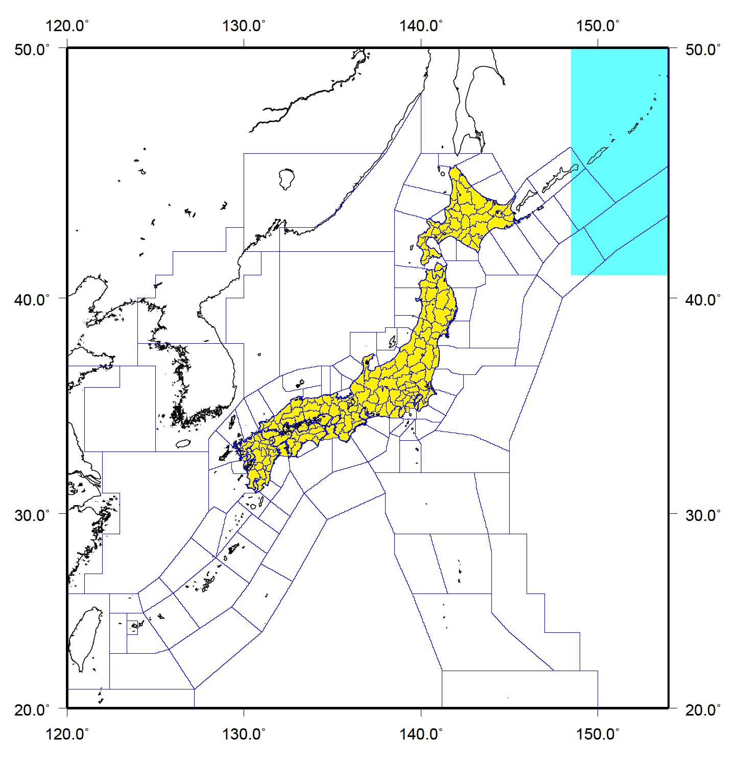 |
| Figure 1: Inland region (yellow part; depth less than 30 km) and region around the Kurile Islands
(aqua-blue part; north of 41 degrees north in latitude and east of 148.5 degrees east in longitude) The blue lines show the boundaries of regions used for Earthquake Information. |
In hypocenter calculation, JMA employs pre-computed tables to determine theoretical travel times between sources and stations. These are created with the assumption of a spherically layered earth model with constant velocities (application since October 1997 outlined below).
From October 1997 to September 2020, the JMA2001 travel time table [Ueno et al. (2002)(3)] was mainly used for theoretical travel time calculation. For earthquakes in the shallow region around the Kurile Islands, the table provided by Ichikawa (1978)(5) was also used, and the Jeffreys-Bullen table (1958)(4)] was used for earthquakes with an epicentral distance of 2,000 km or farther from JMA's seismic network. These tables were calculated assuming a station elevation of 0 m.
On September 1 2020, JMA began using the new ocean bottom seismometers (Seafloor observation network for earthquakes and tsunamis along the Japan Trench (referred to here as the S-net) and Dence Oceanfloor Network system for Earthquakes and Tsunamis (referred to here as the DONET2), where seismic velocity structures differ significantly from those of inland stations, in its hypocenter calculation. Four new travel time tables are now used in line with sub-station seismic velocity structures. JMA2001A is used for inland stations, JMA2020A for those within landward slopes, JMA2020B for those in the outer-rise region of the Japan Trench, and JMA2020C for those in the Nankai Trough area.
The use of these tables in hypocenter calculation enables determination of theoretical travel times between sources and stations at elevations from -4,000 to 3,900 m on land, and from -8,000 to 0 m on the sea bed. For stations with epicentral distances greater than 2,000 km, the time table used until 31 August 2020 continues to be applied(see travel time tables and seismic velocity structure for data).
At OBS stations, observed travel times are behind those based on velocity structures due to an unconsolidated sedimentary layer (P-wave velocity=1.8 km/s, P-wave velocity/S-wave velocity=3.0). JMA uses the procedure reported by Shinohara et al.(2012)(19) to determine station correction for travel times at each station, and applies these corrections in hypocenter calculation (see station correction list file for data).
The maximum amplitude is defined as half of the maximum peak-to-peak amplitude about i~iii.:
In the averaging procedure for ⅰ, ⅱ and ⅲ, the initial mean of magnitudes at all stations
is first calculated. The mean and standard deviation of magnitudes for the stations are then calculated,
with values deviating from the initial mean by more than 0.5 discarded. The mean is adopted as the magnitude
only if the standard deviation is less than 0.35.
The meanings of the symbols used in the above formulas are as follows:
| H | : Focal depth (km) |
| Δ | : Epicentral distance (km) |
| R | : Hypocentral distance(km) |
| α | : Constant 1/0.85=1.176 |
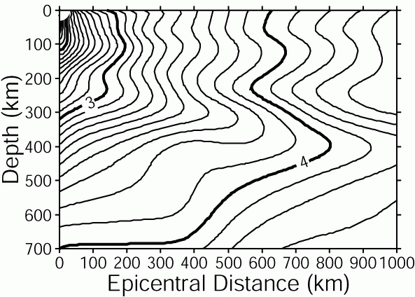
| βD, βV | : Terms showing dependence on Δ and H (see Figure 3 and 4) |
| CD | : Correction value (= 0.2) used for D93-type seismometers |
| CV | : Correction value depending on seismometer types (see Table 1) |
| AN, AE | : Maximum displacement amplitude in the horizontal component of D93-type seismometers. The unit is micrometers = 10−6 m. |
| ASX, ASY, AZY | : Maximum velocity amplitude of the X, Y, and Z observed at the S-net stations The unit is 10−5 m/s. |
| AZ | : Maximum velocity amplitude in the vertical component of EMT-, EMT76- or E93-type seismometers. The unit is 10−5 m/s. |
|
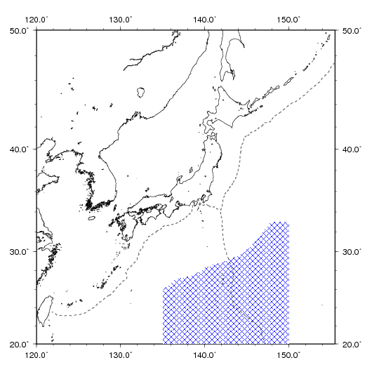
| Figure 2: Region(blue shading) where stations in the ranges of R ≥ 30 km and Δ≤ 2000 km are always used for Displacement Magnitude calculation. |
 |
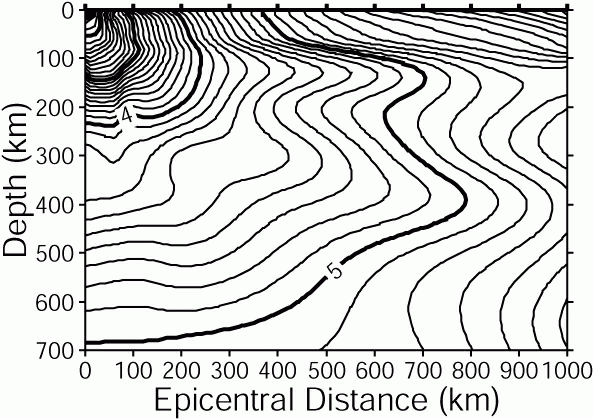 |
| Figure 3 : Contour representation of βD | Figure 4 : Contour representation of βV |
| Seismometer type | Value | Seismometer type | Value |
|---|---|---|---|
| JMA-93 type, velocity sensor, remote, surface installation | 0.00 | JMA velocity sensor, installed in volcanic region | 1.13 |
| JMA OBS, velocity sensor | 0.47 | Other JMA seismometer, velocity sensor | −0.18 |
| JMA-67 type, velocity sensor with logarithmic-amplifier, remote | −0.02 | High-sensitivity seismometer, velocity sensor, bore-hole installation | 0.43 |
| JMA velocity sensor, local, surface installation | −0.02 | Other organization, velocity sensor, ground installation | 0.12 |
| JMA velocity sensor, local, buried | 0.50 | Other organization, velocity sensor, horizontal-tunnel installation | 0.30 |
| JMA velocity sensor with logarithmic-amplifier, local, buried | −0.11 | Other organization, velocity sensor, bore-hole installation | 0.48 |
| JMA velocity sensor, remote, surface installation (except 93 type) | 0.03 | Other organization OBS, velocity sensor(except S-net) | 0.11 |
| S-net, velocity sensor below the sea bed | 0.51 | S-net, velocity sensor on the sea bed | 0.27 |
| JMA velocity sensor, remote, buried | 0.29 |
The Matched Filter (MF) method [Moriwaki (2017)(18)] was introduced in March 22 2018 to enable the detection of deep low-frequency earthquakes occurring on the plate boundary along the Nankai Trough. Automatic hypocenter determination using this approach is based on application of the four-dimensional grid search method near the detected event. If the hypocenter is determined to be at the edge of a grid space, the template event hypocenter is adopted.
Magnitude is calculated as the average of
Mv=Mtemplate+αlog(Az/Aztemplate)
Here:
| α | :Constant 1/0.85=1.176 |
| Mtemplate | :Magnitudes of the template for low-frequency earthquakes |
| Az,Aztemplate | :Maximum velocity amplitude in the vertical component of detected and template low-frequency earthquakes |
The notation of the magnitude determined is Mv regardless of the number of stations used for determination.
A new auto hypocenter detection approach (the PF method; [Tamaribuchi et al. (2016)(17)]) was adopted in April 2016, and three new hypocenter categories were introduced.
The distribution of Mth values is shown Figure 5. The number is 1.7 on and near land, increasing to 3.5 with distance from land.
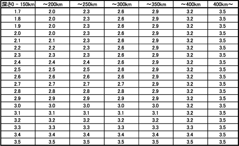
For earthquakes occurring deeper than 150 km, Mth increases as shown in Table 2. For the prediction of the Tokai Earthquake, Mth for the Tokai area is smaller than conventionally set in other areas for all depths, as shown Figure 6. However, based on examination to determine the precision of results from automatic processing using the PF method, Mth values were unified on March 22, 2018.
The hypocenter determined using the MF method is always classified as C as shown above regardless of Mth values.
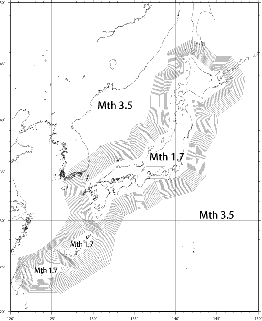 |
| Figure 5: Mth distribution (at depths from 0 to 150 km), with solid lines representing increments of 0.1 except in the Tokai district. |
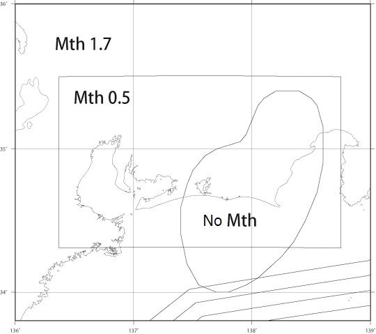 |
| Figure 6: Mth for the Tokai district (Until March 21,2018) |
| Table 2: Mth with depth |
 |
If more than 40 stations report observation in fully checked hypocenter classification, the 40 nearest the focus are used for calculation (as of October 1997) [Earthquake Prediction Information Division, Seismology and Volcanology Department, Japan Meteorological Agency (1998)(6)]. Stations are selected as outlined below.
In simply checked hypocenter classification, all available stations are used for calculation.
In automatic hypocenter classification, the selection applied in fully checked hypocenter categorization is performed only with the PF method.
The calculated earthquake parameters are categorized into classes K, S, k, s, A and a based on their accuracy and determination methods.
| High-precision hypocenters | Low-precision hypocenters | |||
|---|---|---|---|---|
| Over Mth | K (fully checked) | S (fully checked) | ||
| Less than Mth | k (simply cheked) | A (Auto) | s (simply cheked) | a (Auto) |
Full checking is performed for earthquakes with a seismic intensity of 1 or more in Japan, and otherwise where necessary.
The hypocenter classification standards are outlined below. The inland region is defined as shown in Figure 1, and the general region is defined as all areas except the inland region and the region around the Kurile Islands.The hypocenter determined using the MF method is classified as "a (Auto)" as shown above regardless of accuracy.
| High-precision hypocenters (K, k, A) | |||
|---|---|---|---|
| Region | Inland | General | Region around the Kurile Islands |
| Origin time error | Less than 0.5 sec | Less than 1.0 sec | Less than 1.5 sec |
| Epicenter latitude/longitude estimation error | Less than 3.0 min | Less than 5.0 min | Less than 10.0 min |
| Low-precision hypocenters (S, s, a) | |||
|---|---|---|---|
| Region | Inland | General | Region around the Kurile Islands |
| Origin time error | 0.5 – 2.0 sec | 1.0 – 2.0 sec | 1.5 – 2.0 sec |
| Epicenter latitude/longitude estimation error | 3.0 – 10.0 min | 5.0 – 10.0 min | 10.0 – 15.0 min |
This bulletin lists class-K, k and A hypocenters only.
Earthquake* parameters and data on wave arrival at the seismic stations of JMA and other organizations** are listed.
* Earthquakes included on this list meet at least one of the following conditions:
— JMA calculates the hypocenter and magnitude
— USGS calculates the hypocenter and mb or Ms as about 6 or greater, or the tremor is felt at a Japanese station
(a JMA seismic intensity of 1 or larger).
** National Research Institute for Earth Science and Disaster Prevention, Hokkaido Univ., Hirosaki Univ., Tohoku Univ., The Univ. of Tokyo, Nagoya Univ., Kyoto Univ., Kochi Univ., Kyushu Univ., Kagoshima Univ., the National Institute of Advanced Industrial Science and Technology, the Geospatial Information Authority of Japan, the Japan Agency for Marine-Earth Science and Technology, Association for the Development of Earthquake Prediction, Aomori Pref., the Tokyo Metropolitan Government, Shizuoka Pref., the Hot Springs Research Institute of Kanagawa Prefecture, EarthScope Consortium
Estimated focal parameters are shown at the top of the field assigned to each event. For hypocenters with a fixed focal depth, the symbol (F) is shown after the focal depth value. Focal data with large estimation errors are reported as "POOR SOLUTION" and are excluded from 1.2 Earthquake parameters. For hypocenters determined using the MF method, the notation "MF" is placed in the first line. Template event information is also shown below the focal parameters. For distant earthquakes, parameters provided by other organizations such as USGS are included in the table. The notation "AFTER USGS" is placed in the first line in such cases. However, the Mw value based on JMA's centroid moment tensor solution may alternatively be given as the magnitude. Arrival parameters observed at each station are listed in order of epicentral distance. Arrival data on earthquakes whose focal parameters cannot be determined are given in order of the observed arrival time.
For earthquakes whose nodal plane solution or CMT solution is determined, information on the solution is shown below the focal parameters.
Any special remarks or extra information on matters such as damage and/or tsunami heights are included under "REMARK."
| where | ||
| th: | Epicentral angular distance (in radian) | |
| phE lE: | Geocentric latitude and longitude of epicenter | |
| phS lS: | Geocentric latitude and longitude of station |
| where | ||
| Δ: | Epicentral distance (km) | |
| r: | Average radius of the earth (6,371.009km) |
For data on events detected using the MF method, column details are as follows:
Monthly and annual epicenter distributions are shown in the figures titled "Earthquake epicenters in Japan and adjacent regions" and "Regional distribution of earthquakes." Annual distributions of epicenters within certain depth layers are also shown.
Nodal plane solutions for major earthquakes are shown using lower-hemisphere equal-area projection. The values of their solution parameters, the strike (STR), dip (DIP) and slip-direction (SLIP) of nodal planes (NP1, NP2), and the azimuth (AZM) and plunge (PLG) of the P-, T- and N-axes are shown under each figure. The strike of each plane and the azimuth of each axis are measured clockwise from north. The dip of each plane and the plunge of each axis are measured downward from the horizontal plane. Slip signifies the motion of a hanging wall relative to a foot wall, and its direction is measured counterclockwise from the strike direction. Nodal plane solutions are determined using the method of Nakamura and Mochizuki(1998)(10), and take-off angles are calculated based on the velocity structure of Ueno et al.(2002)(3) Since September 2020, the take-off angle at OBS stations has been calculated using JMA2020A, JMA2020B and JMA2020C (see take-off angle table and seismic velocity structure).
CMT solutions for major earthquakes are shown using lower-hemisphere equal-area projection. The CMT solution determination method is based on Kawakatsu (1989)(11). For further details, see Nakamura et al. (2003)(12).
Information on each CMT solution is shown above and below the figure as follows:
| 1st line | : Origin time (JST) |
| 2nd line | : Region name |
| Hypo. | : Location (latitude, longitude, depth) of hypocenter |
| Cent. | : Location (latitude, longitude, depth) of centroid |
| Δ t | : Centroid time minus origin time (sec.) |
| Mo | : Scalar momentt |
| Mw | : Moment magnitude |
| Mj | : JMA magnitude |
| mrr,mtt,mff,mrt,mrf,mtf | : Moment tensor components |
| STR | : Strike of nodal planes (NP1, NP2) |
| DIP | : Dip angle of nodal planes (NP1, NP2) |
| SLIP | : Slip angle of nodal planes (NP1, NP2) |
| MOM | : Moment tensor component of P-, T- and N-axes |
| AZM | : Azimuth of P-, T- and N-axes |
| PLG | : Plunge of P-, T- and N-axes |
| V.R. | : Variance reduction |
| ε | : Non-double couple component ratio |
| N | : Number of stations used |
| COMP | : Number of components used |
The moment tensor is expressed by the spherical polar coordinates (r, t, f), which represent upward, southward and eastward positive respectively.
The strike of each nodal plane and the azimuth of each axis are measured clockwise from north. The dip of each nodal plane and the plunge of each axis are measured downward from the horizontal plane. Slip signifies the motion of a hanging wall relative to a foot wall, and its direction is measured counterclockwise from the strike direction.
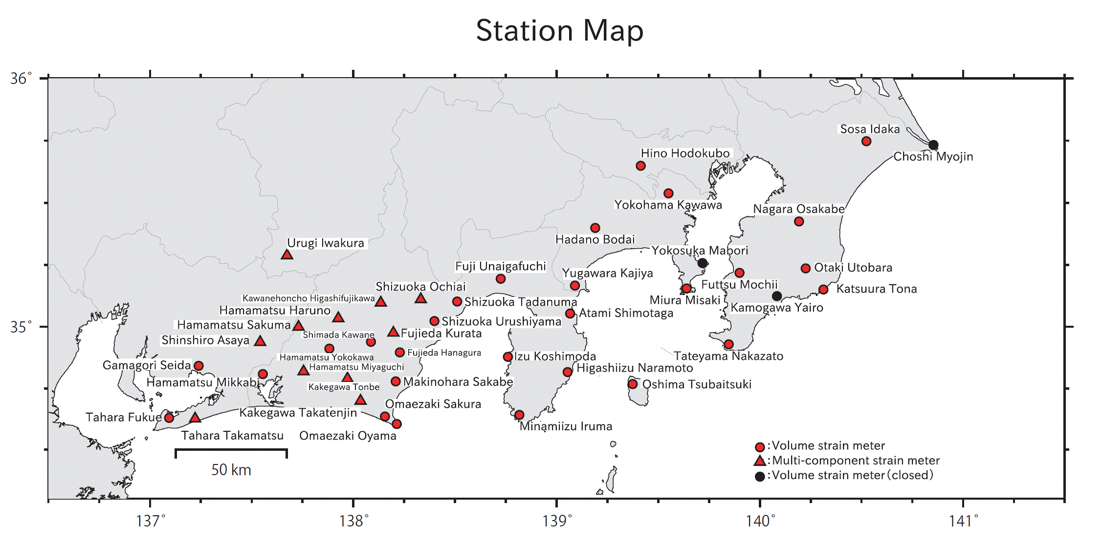
Dilatational strain is continuously observed using borehole strain meters [Seismological Division, Observation Department (1979)(13), Nihei et al. (1987)(14)] and multi-component strainmeters [Ishii et al. (1992)(15)] in the Tokai and southern Kanto regions. The "Volume strain observation stations" and "Linear strain observation stations" tables in Appendix 2.A give station names, station codes, latitudes, longitudes, altitudes and depths of strain meters. The "Directions of measurement" table in Appendix 2.A gives sensor names and directions of measurement. The distribution of stations is shown in the figure "Crustal strain station map".
The data consist of hourly means of strain values. Positive and negative values correspond
to crustal expansion and contraction, respectively, relative to the value at the time when observation
was started.
An asterisk indicates that the value has been modified from the original. Some values are
accompanied by one of the following:
| LOSS | Loss of data |
| V.O. | Valve Open |
| I | Instrumental adjustment |
| P | Power failure |
| O | Others |
The data consist of hourly means of linear strain for each component.
Positive and negative values correspond to crustal expansion and contraction, respectively,
relative to the value at the time when observation was started.
An asterisk indicates that the value has been modified from the original.
Some values are accompanied by one of the following:
| LOSS | Loss of data |
| Z.S. | Zero Shift |
| I | Instrumental adjustment |
| P | Power failure |
| O | Others |