El Niño Monitoring and Outlook

• Table) El Niño Monitoring Indices
• Fig.3) Time series of sea surface temperature (SST) deviations for NINO.3, NINO.WEST, and IOBW, and the Southern Oscillation Index.
• Fig.4) Monthly mean SST and anomalies in the Pacific and Indian Oceans.
• Fig.5) Depth-longitude cross sections of temperatures and anomalies along the equator in the Indian and Pacific Oceans by ocean data assimilation system.
• Fig.6) Time-longitude cross section of SST anomalies along the equator in the Indian and Pacific Oceans.
• Fig.7) Time-longitude cross section of ocean heat content (OHC; vertically averaged temperature in the top 300 m) anomalies.
• Fig.8) OLR and Equatorial Zonal Wind Indices.
• Fig.9) Monthly-mean Outgoing Longwave Radiation (OLR) and anomalies.
• Fig.10) Time-longitude cross sections of velocity potential anomalies at 200 hPa and zonal wind anomalies at 850 hPa along the equator.

• Fig.11) Outlook of the SST deviation for NINO.3 by the seasonal ensemble prediction system.
• Fig.12) Outlook of the SST deviation for NINO.WEST by the seasonal ensemble prediction system.
• Fig.13) Outlook of the SST deviation for IOBW by the seasonal ensemble prediction system.

El Niño Outlook

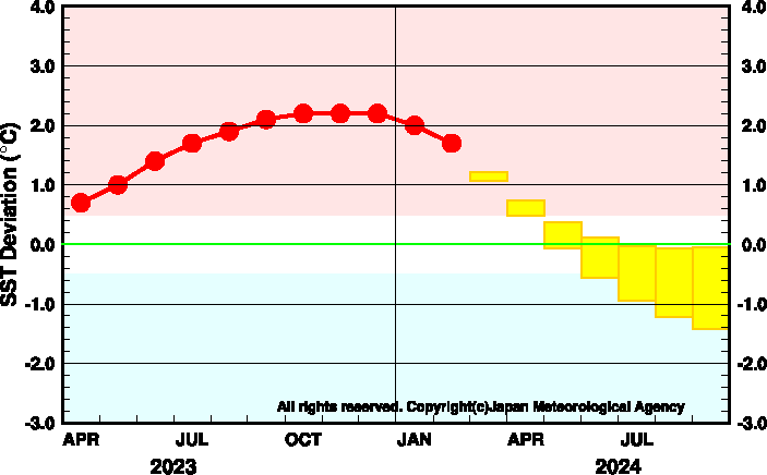
Fig.1 Five-month running mean of the SST deviation for NINO.3 predicted by JMA's seasonal ensemble prediction system (JMA/MRI-CPS3).

Red dots indicate observed values, and boxes indicate predictions. Each box denotes the range where the value will be included with the probability of 70%.

YEAR	MONTH	mean period
2024	NOV	SEP2024–JAN2025
	DEC	OCT2024–FEB2025
2025	JAN	NOV2024–MAR2025
	FEB	DEC2024–APR2025
	MAR	JAN2025–MAY2025
	APR	FEB2025–JUN2025
	MAY	MAR2025–JUL2025
El Niño ENSO neutral La Niña

Fig.2 ENSO forecast probabilities based on JMA/MRI-CPS3.

Red, yellow, and blue bars indicate probabilities that the five-month running mean of NINO.3 SST deviation from the latest sliding 30-year mean is +0.5°C or above (El Niño), between +0.4°C and -0.4°C (ENSO Neutral), and -0.5°C or below (La Niña), respectively. Labels in lightface indicate the past months, and ones in bold face indicate the current and future months.

El Niño Monitoring

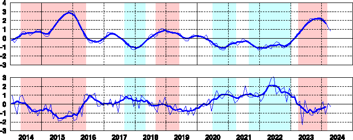
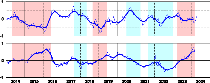
Fig.3 Time series of sea surface temperature (SST) deviations from the climatological mean based on the latest sliding 30-year period for NINO.3, (the 2nd panel), Southern Oscillation Index (the 3rd panel), SST deviations for NINO.WEST (the 4th panel), and SST deviations for IOBW (the bottom panel). (each region is shown in the top panel).

Thin lines indicate a monthly mean value, and smoothed thick curves, a five-month running mean. Red shaded areas denote El Niño periods, and blue, La Niña ones.

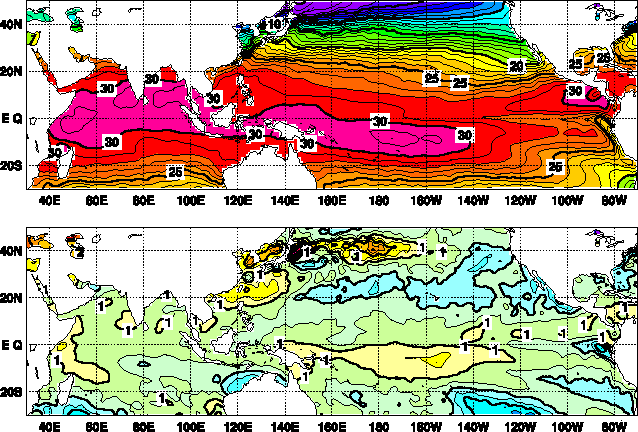
Fig.4 Monthly mean SST and anomalies in the Pacific and Indian Oceans. Base period for normal is 1991-2020.

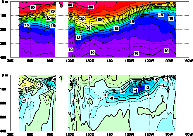
Fig.5 Depth-longitude cross sections of temperature and anomalies along the equator in the Indian and Pacific Oceans by the ocean data assimilation system. Base period for normal is 1991-2020.

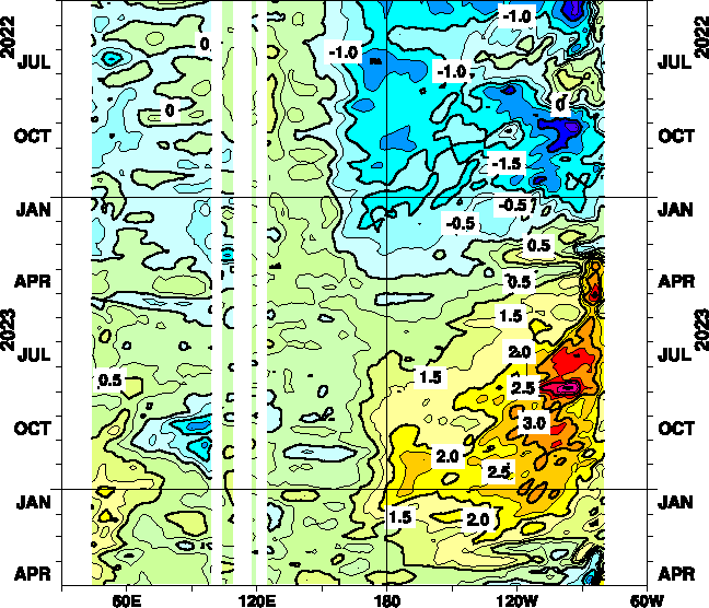
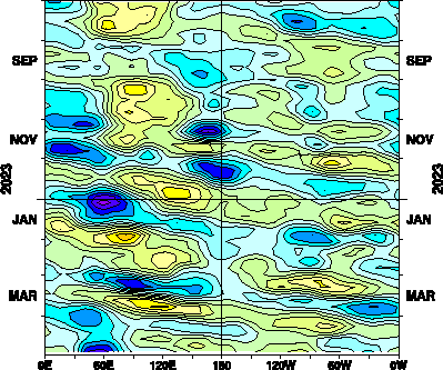
Fig.6 Time-longitude cross section of SST anomalies along the equator in the Indian and Pacific Oceans. Base period for normal is 1991-2020.

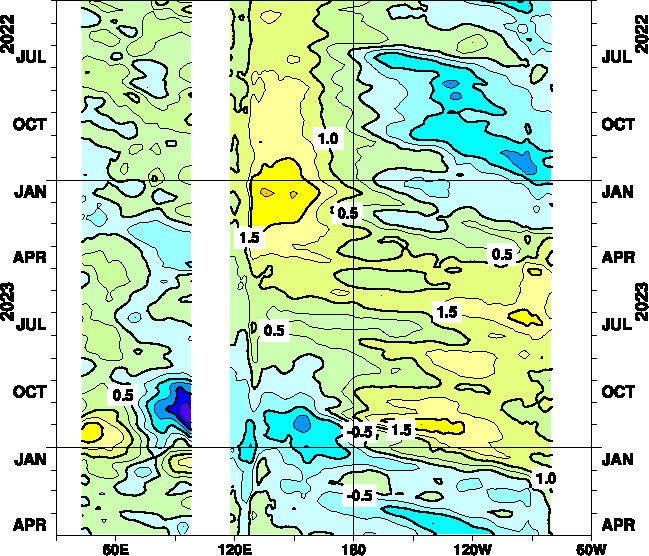
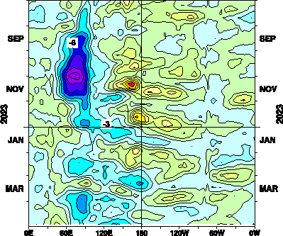
Fig.7 Time-longitude cross section of ocean heat content (OHC; vertically averaged temperature in the top 300 m) anomalies along the equator in the Indian and Pacific Oceans by the ocean data assimilation system. Base period for normal is 1991-2020.

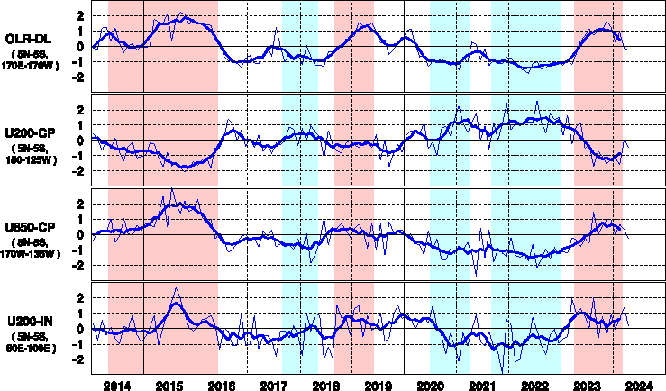
Fig.8 Time series of OLR index around the International Date Line (OLR-DL), equatorial zonal wind index at 200 hPa in the central Pacific (U200-CP), equatorial zonal wind index at 850 hPa in the central Pacific (U850-CP), and equatorial zonal wind index at 200hPa in the Indian Ocean (U200-IN) (from upper to lower). Base period for normal is 1991-2020. Red shaded areas denote El Niño periods, and blue, La Niña ones. Original OLR data were provided by NOAA. (Notice: OLR data were replaced with the new NOAA CPC Blended OLR data provided by NOAA/CPC in October 2023.)

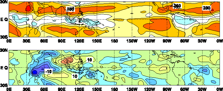
Fig.9 Monthly mean outgoing longwave radiation (OLR) and anomalies. Base period for normal is 1991-2020. Original data were provided by NOAA. (Notice: OLR data were replaced with the new NOAA CPC Blended OLR data provided by NOAA/CPC in October 2023.)

Fig.10 Time-longitude cross sections of velocity potential anomalies at 200 hPa (left) and zonal wind anomalies at 850 hPa (right) along the equator. Base period for normal is 1991-2020.

Model Predictions of ENSO monitoring indices

These figures indicate a time series of the monthly sea surface temperature (SST) deviation for NINO.3 (5°N-5°S, 150°W-90°W), NINO.WEST (10°N-EQ, 130°E-150°E), and IOBW (20°N-20°S, 40°E-100°E). Thick line with closed circle shows the observed SST deviation and boxes show the predicted one for the next six months by the seasonal ensemble prediction system. Each box denotes the range where the SST deviation will be included with the probability of 70%.

Fig.11 Outlook of the SST deviation for NINO.3 by the seasonal ensemble prediction system.

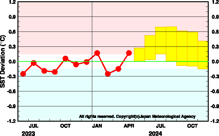
Fig.12 Outlook of the SST deviation for NINO.WEST by the seasonal ensemble prediction system.

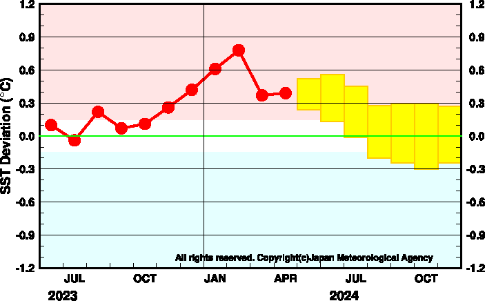
Fig.13 Outlook of the SST deviation for IOBW by the seasonal ensemble prediction system.